Imagine you’re on a quest to find the minimum of something, but you’re like a fish in a labyrinth. All you know is that somewhere out there lies a minimum hiding away. You’re blind to whether the function is friendly enough to be differentiable (No Gradient Descent, my old friend), and oblivious to potential divergences.

So, what’s your only option? It seems like touching the function with a stick and observing its reaction is the way to go.

Take, for instance, a simple 2-slot function creatively named ‘hidden’:

def hidden(a, b):
    # a and b in [0,1000]
    something = some calculations that depend on a, b
    return something

You roll up your sleeves and embark on what can only be described as a game of trial and error. Want the minimum? Roll the dice and try every conceivable combination of x and y — a strategy known as the Grid Search. But it’s like searching for a needle in a haystack. But hey, it works! If you live more than he universe…
Let’s see why.

Let me define the ‘super_hidden’ function:

def super_hidden(a, b, c, d, e, f, g, h, i, j, k, l):
    # a, b, c, d, e, f, g, h, i, j, k, l in [0,1000]
    somethingElse = some calculations that depend on a, b, c, d, e, f, g, h, i, j, k, l
    return somethingElse

Ready to tackle it with Grid Search? Think again.

Picture this: the function is so complex that it takes a solid second just to spit out a result for a random mishmash of parameters. With $1000^{12} \approx 10^{36}$ possible combinations, is a lot of years.

What could be a good solution to this problem? Genetic Algorithms

Genetic Algorithms

Genetic algorithms are a class of optimization algorithms inspired by the process of natural selection and genetics. They are commonly used to solve complex problems that involve finding the best solution among a large set of possibilities.

The basic idea behind genetic algorithms is to mimic the process of evolution by iteratively generating a population of candidate solutions, evaluating their fitness, and applying genetic operators such as selection, crossover, and mutation to create new generations of solutions.

Over time, the algorithm (should) converges towards the optimal solution.

The best part? The best part is that every element of a new generation is completely independent from the other and guess who can play a role here? Multithreading.

The Toy Genetic Algorithm

I’ve implemented a version of Genetic Algorithm grasping knowledge from here and there and the fun part is that seems to have sense and converges.

Let’s split up the problem.

1. Fitness Function

The fitness function determines how “fit” an individual is within the population. Basically, for the problem of minimizing a function, like the hidden function, it assesses how good the parameters chosen to evaluate the function are. If the function yields a considerably smaller absolute value compared to the previous one for a particular choice of parameters, then you are getting closer to a minimum.

Let’s define the fitness function.

def f(X,Y):
    Z = ((X-500)**2 - 100000 * np.cos(2 * np.pi * X)) + ((Y-500)**2 - 100000 * np.cos(2 * np.pi * Y)) + 20
    return Z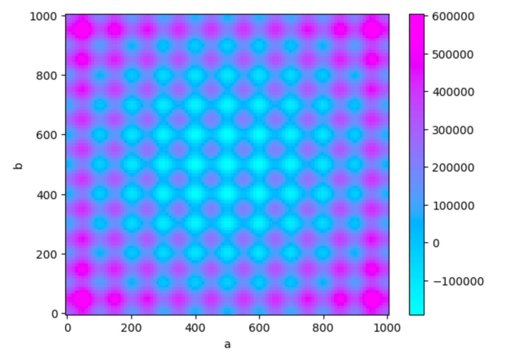

This function is called Rastrigin function and is often used when exploring numerical optimization because it has a lot of local mnima and in the middle it has a global minimum.

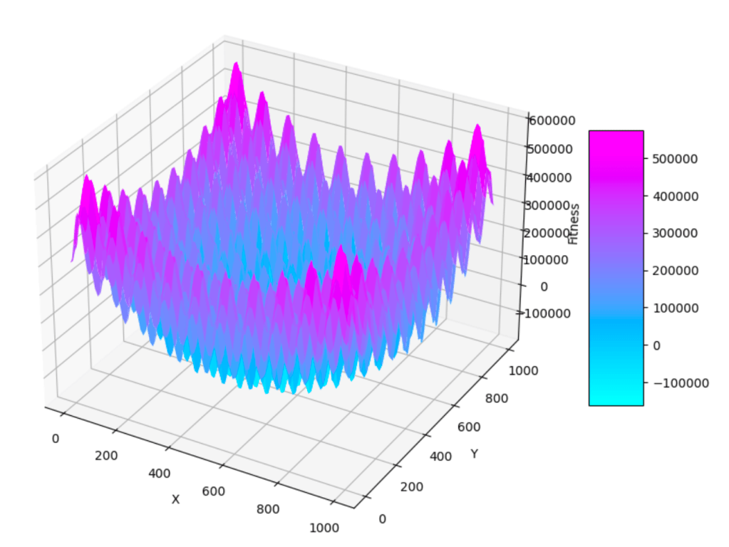
In 3D this function looks like this

Now let’s delve deep into the algorithm.

2. Encoding and Scaling

The second step involves creating a genetic code for each member of the population. This genetic code essentially represents the values of the parameters that our hidden function relies on. There are several ways to accomplish this, but I opted for a method where I convert the value of each parameter into a binary format.

• Encoding: We take a real number value and scale it to fit within a specified range. Then, we convert this scaled value into a binary representation using a fixed number of bits.
• Decoding: Decoding, on the other hand, reverses the encoding process by converting the binary strings back into their original parameter values.

Now, you might be wondering why I choose this specific approach.

Imagine an example in which your parameters vary from 0 to $10^{-10}$.
If we were to express these values in a floating-point representation, we’d allocate space for both the exponent and the mantissa. However, in our algorithm, mutations occur at some point, and if a mutation affects the part of the DNA where the exponent is encoded, it could drastically alter the magnitude of the number, which isn’t ideal.

To address this, I’ve implemented a controlled mutation strategy using 10 bits and the minimum and maximum values of the parameter for encoding. By doing so, mutations affect these 10 bits ensuring changes stay within the specified range.

def encode_and_scale(real_value, min_value, max_value, num_bits):
    scaled_value = int((real_value - min_value) / (max_value - min_value)    (2**num_bits - 1))
    binary_representation = bin(scaled_value)[2:].zfill(num_bits)

    return binary_representation



def decode_and_rescale(encoded_value, min_value, max_value, num_bits):
    scaled_value = int(encoded_value, 2)
    real_value = min_value + scaled_value / (2**num_bits - 1) * (max_value - min_value)

    return real_value

3. Initialization

The algorithm require some inizilization value such as population size, number of children, probabilities of crossover and mutation, and the number of evaluations. It also sets the range for two variables, a and b, which will be optimized using the genetic algorithm.

num_parameters = 2
population_size = 6
num_childs = 4 #not necessary
pc = 0.6 # Probability of crossover
pm = 0.03 # Probability of mutation

And here the ranges

a, a_MAX, a_MIN = 46, 0, 1000
b, b_MAX, b_MIN = 678, 0, 1000

4. Population Initialization

The InitPopulation function initializes the population by randomly generating values for a and b (in between the ranges). It calculates the fitness of each individual using a fitness function and stores the encoded values and fitness in a dictionary

# Initialize the population
def InitPopulation():
	generations = {}
	for i in range(population_size):
		random_a = random.uniform(a_MIN, a_MAX)
		random_b = random.uniform(b_MIN, b_MAX)

		fit = fitness(random_a, random_b)
		a_bin = encode_and_scale(random_a, a_MIN, a_MAX, 10)
		b_bin = encode_and_scale(random_b, b_MIN, b_MAX, 10)

		dna = a_bin + b_bin
		generations[i] = {"dna": dna, "fitness": fit}

    return generations

5. Selection: Roulette Wheel

The roulette_wheel function implements the selection operation using the roulette wheel method.
It’s an important part because here we decide who survives and who dies.
Powerful right?

Basically it computes the selection probabilities for each individual based on their fitness and creates a cumulative probability distribution. It then randomly selects individuals based on their cumulative probabilities to form the new generation.

Imagine we have a group of individuals, each with a different fitness. We want to select individuals from this group to form a new generation.

Here’s how the roulette wheel works:

1. Assigning Probabilities: We give each individual a slice of a spinning wheel based on their fitness. The fitter they are, the bigger their slice.
2. Spinning the Wheel: Now, imagine spinning this wheel. It stops randomly at a certain point.
3. Selecting an Individual: Wherever it stops, we pick the individual whose slice includes the point where the wheel stopped. So, if the wheel stopped in a big slice, we’d pick the fitter person associated with that slice.
4. Repeating the Process: We repeat this spinning and selection process multiple times to pick several individuals for our new generation.

def roulette_wheel(generationDictN):

	total_fitness = sum(individual["fitness"] for individual in generationDictN.values())
	
	if total_fitness == 0: #could have been done better, I know 
		return generationDictN
	
	selection_probabilities = {key: individual["fitness"] / total_fitness for key, individual in generationDictN.items()}
	
	cumulative_probabilities = {}
	cumulative_prob = 0
	
	for key, prob in selection_probabilities.items():
		cumulative_prob += prob
		cumulative_probabilities[key] = cumulative_prob
	
	new_generation = {}
	
	for _ in range(len(generationDictN)):
		rand_num = random.random()
		selected_key = next(key for key, prob in cumulative_probabilities.items() if prob >= rand_num)
	
		new_generation[_] = generationDictN[selected_key]
	
	return new_generation

Mutation function

The Mutation function applies mutation to each individual in the population. It randomly flips bits in the binary string representation of an individual with a certain probability.

# Mutation function

def Mutation(individual):

	encoded_value = individual["dna"]

	mutated_encoded_value = ''.join(
	'0' if bit == '1' and random.random() < pm
	else '1' if bit == '0' and random.random() < pm 
	else bit 
	for bit in encoded_value
	)

	individual["dna"] = mutated_encoded_value

	return individual

This was version 1, but then someone made me realize that there might be a problem with this mutation function.

Indeed in our conversion, there are 10 bits, but they do not carry the same importance. For example, flipping the first bit can significantly change the parameter, whereas flipping the last bit might not have as much impact. Therefore, we need a mutation approach that addresses this issue.

# Mutation function

def flip_bit(bit):
	return '1' if bit == '0' else '0'
	
def Mutation(individual, num_bits=10):
	encoded_value = individual["dna"]
	mutated_encoded_value = ''
	
	nb = 0
	for i, bit in enumerate(encoded_value):
		nb = nb + 1
		
		# Exponential decay function for mutation probability
		mutation_prob = np.exp(-0.5 * nb) * pm 
		rm = random.random()
		if rm < mutation_prob:
			mutated_bit = flip_bit(bit)
		else:
			mutated_bit = bit
		
		mutated_encoded_value += mutated_bit
		if nb == num_bits:
			nb = 0
	
	individual["dna"] = mutated_encoded_value
	return individual

I’ve defined an exponential decay probability function, which means flipping the first bit (that encodes higher values) is less likely than flipping one of the last bits, which don’t change the parameter as much.

It’s better like this.

8. Decoding and Fitness Calculation

The `DecodeAndCalFitness` function decodes the binary strings of the selected individuals back into real values for `a` and `b`. It calculates the fitness of each individual using a fitness function and updates their fitness values in the population dictionary. It also saves the best fitness and the iteration in which it has been found.

Additionally, the code creates a CSV file with the parameters and the fitness every time the fitness function has been computed, just to observe how the parameters evolve over time.

for _, individual in SelectedNumbersDict.items():

    num = individual["dna"]
    variables = [num[i:i+10] for i in range(0, len(num), 10)]
    a, b = variables

    map_a = decode_and_rescale(a, a_MIN, a_MAX, 10)
    map_b = decode_and_rescale(b, b_MIN, b_MAX, 10)

    fit = fitness(map_a, map_b)
    individual["fitness"] = fit

    with open('ToyValues.csv', 'a') as f:
        f.write(f'{map_a},{map_b},{fit}\n')

    if fit < bestfit:
        bestfit = fit
        bestXY = num

return SelectedNumbersDict, bestfit, bestXY

10. Run the algorithm

Finally, you loop over the number of generations that you want and wait.

# Genetic Algorithm

def GA():

	t = 0
	bestfitness = 0 # Initialize to positive infinity
	bestXY = ""
	IterFound = 0
	generationDictN = InitPopulation()

	print("InitPop", generationDictN)
	
	while t < maxIteration:
	
		print("Generation: ", t , "-----------------")
		SelectedNumbersDict = roulette_wheel(generationDictN)
		print("Roulette", SelectedNumbersDict)
		SelectedNumbersDict = CrossOver(SelectedNumbersDict)
		print("Crossover", SelectedNumbersDict)
		SelectedNumbersDict = {key: Mutation(individual) for key, individual in SelectedNumbersDict.items()}
		print("Mutation", SelectedNumbersDict)
		generationDictN, bestfit, bestXandY = DecodeAndCalFitness(SelectedNumbersDict)
		
		if bestfit < bestfitness:
			bestfitness = bestfit
			bestXY = $bestXandY$
			IterFound = t
			t += 1
			
	return bestfitness, bestXY, IterFound
	
	
	bestfitness, bestXY, IterFound = GA()

Conclusion

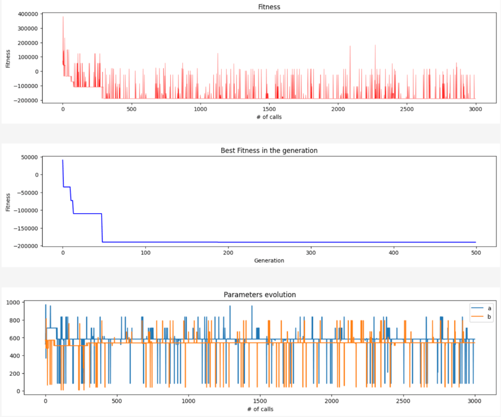
After a little bit we find

Best Fitness: -190179.21226216253
Mapped a: 583.9941348973607
Mapped b: 542.9794721407625 
Iteration Found: 188

To understand the algorithm’s operations, we can observe the “tried” configuration of parameters represented in black, while the red dot denotes the final value, which serves as the output of the algorithm.

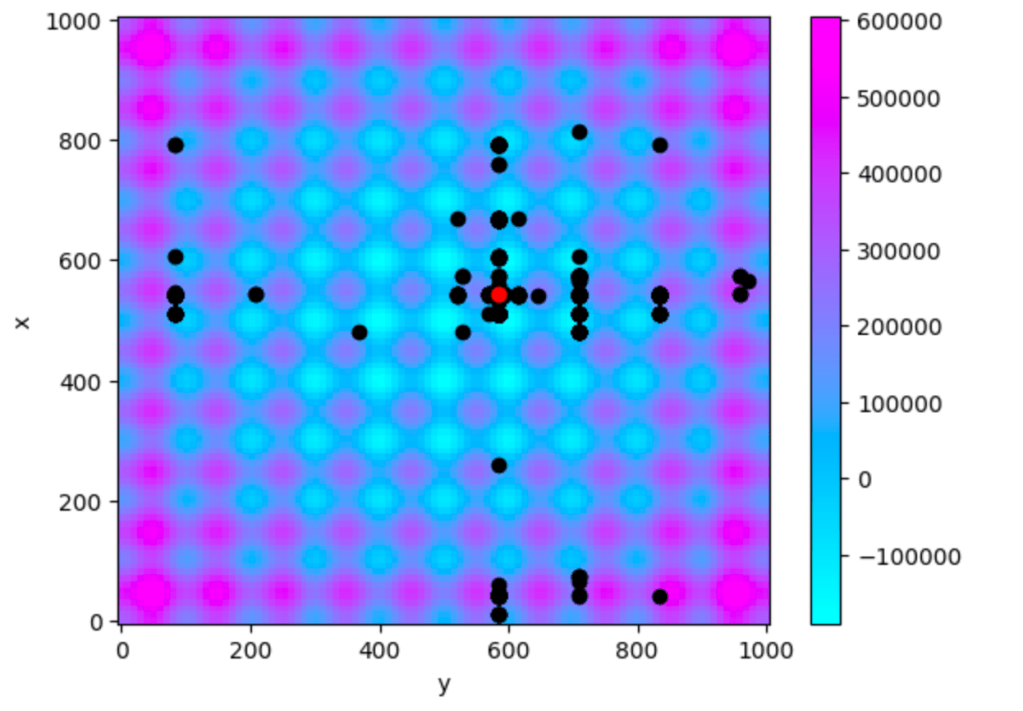
It’s worth noting that not all possible combinations of parameters have been tried. Even if there are some blind spots where the function has not been evaluated, we have achieved a remarkably good result, approaching the minimum, which is satisfactory. Also the reslut is similar every time we find the run the algorithm.

Here the evolution of the fitness every time that has been called (in red), in blue the best value of the fitness for every generation and the last plot is the evolution of the parameters.

Side note

This implementation reflects my personal fascination with this particular algorithm. While I acknowledge the existence of many effective genetic algorithms, I felt inspired to build this one from scratch.
The entire source code is available on GitHub and I would be thrilled if others wished to contribute. If you have ideas for improving the algorithm or wish to propose changes, feel free to fork the repository and submit your pull requests.